Interleaved Projected Gradient Descent for Safe Imitation Learning

Shengfan Cao; Francesco Borrelli

Preprint 2026 / Safe imitation learning

InterleavedProjected Gradient Descent
for Safe Imitation Learning

Imitate the expert.
Then correct toward safety.

Training alternates one imitation step with a block of safety steps that pull the network’s actions toward their projection onto the safe set. At run time, the controller is the network alone, with no safety filter.

Shengfan Cao · Francesco Borrelli

Read the paper ↗ Try the toy problem ↓

Conceptual diagram in policy-output space: an imitation step moves the actions toward the demonstrations and outside the safe set; a block of safety steps pulls them back to its boundary. — **Interleaveimitation steps with safety blocks**Conceptual illustration

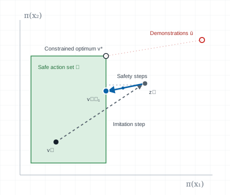
01 / ImitateOne gradient step on the cloning loss

02 / CorrectA block of steps toward projected actions

03 / DeployThe network alone, with no filter

The question

Can the safety filter make
the policy safer to begin with?

A projection-based safety filter can wrap any policy. But an unsafe policy triggers frequent or large interventions, and while the filter stays active, the closed loop drifts from the intended behavior.

We use the filter during training instead. Imitation and safety correction stay separate operations: one imitation gradient step, then a block of safety steps that regress the network’s actions toward their projection onto the safe set.

Most alternatives add a weighted safety penalty to the imitation loss. That weight sets the safety–performance trade-off and has to be tuned for each problem. Interleaving needs a safety budget that is only large enough.

Explore the geometry

Interleaving against
a fused penalty.

One training state with a two-dimensional action, so the policy’s output is a point in the plane and the safe action set is an ellipse. The demonstrated action lies outside it. Both methods start from the same output and see only the imitation gradient and projections of their own actions. Neither is told the constrained optimum v*.

Fused penalty weight λ 1

Fused step size

Coupling between the two outputs 0.30

Press Play animation to watch both policies train from the same start, one step at a time.

An affine toy of Sections III–IV. Interleaving follows a recipe that converges well here: refreshed safety targets, a safety block of K_t = ⌈ln(t + 2)⌉ steps, a learning rate that decays from 0.2 to 0.002 over the run, and safety steps near their stability limit. The run lasts 80 (1 + h)/(1 − h) iterations: stronger parameter sharing makes the problem worse conditioned, so it needs longer. Fused training shares the same learning rate. The weight λ only affects fused training; interleaving has no weight to tune.

Safe actions Demonstrations Constrained optimum Interleaved Fused penalty Projection target

Outer iteration t of 1490Next block: K₀ = 1 safety step

Learning rate ηₜ—Decays from 0.2 to 0.002

Predicted fused bias—Distance ‖∇ℓ‖/λ to 𝒞

Safety-step distortion—κ_S, largest tilt from the outward normal

Where each policy is now
Method	Distance to 𝒞	Distance to v*	Gradient steps
Interleaved	—	—	—
Fused penalty	—	—	—

What is computed in this example?

The output is the action v = π(x) = (u₁, u₂) at a single training state, with safe set 𝒞 = {u : u₁²/1.2² + u₂²/0.9² ≤ 1}. Projection onto the ellipse has no closed form; it is computed from its optimality conditions with a one-dimensional bisection. The demonstration is ū = (1.9, 0.5), so the constrained optimum is v* = Π_𝒞(ū) ≈ (1.16, 0.23). The policy is affine in its weights with neural-tangent-kernel Gram matrix H = [[1, h], [h, 1]]; the coupling slider sets h, which models weights shared by the two outputs.

Interleaved: v ← v − η_tH(v − ū), then K_t = ⌈ln(t + 2)⌉ times v ← v − βH(v − Π_𝒞(v))

Fused: v ← v − η_f H[(v − ū) + λ(v − Π_𝒞(v))]

The learning rate decays geometrically, η_t = 0.2 · 0.01^t/T over a run of T = 80(1 + h)/(1 − h) iterations, and the safety step is β = 0.9/(1 + h), just inside its stability limit 1/‖H‖. The horizon grows with the condition number (1 + h)/(1 − h) of H, because the imitation step converges at rate η(1 − h) along H’s weak direction. The safety schedule is the logarithmic one of Algorithm 1 and Example 1 with c = 1, so the projection error left by each block shrinks over training (Corollary 1). Fused training uses either the shared rate η_f = η_t or the normalized rate η_f = η_t/(1 + λ). Its update is stable only while η_f(1 + λ)(1 + h) < 2, the stability condition of Section IV. With the shared rate, a large λ breaks that condition early in training: each penalty correction overshoots deep into the safe set, and the actions chatter at the boundary until the rate has decayed. Normalizing the rate keeps it stable but divides the imitation step by 1 + λ, as in the “Fused, η/(1 + λ)” row of the racing ablations.

The fused update descends ℓ + λφ, a quadratic penalty. Since φ has zero gradient on the safe set, v* is never a stationary point of it, and the fused outputs settle outside 𝒞 at distance ‖∇ℓ‖/λ. Raising λ shrinks that bias, but then the shared rate overshoots and the normalized rate slows imitation; no learning-rate schedule moves the fixed point. With h > 0, each safety step is tilted away from the outward normal of the ellipse; the largest tilt is the distortion κ_S of Assumption 2. On the curved boundary this leaves interleaving an offset from v* proportional to the learning rate, which the decaying rate removes. With a constant rate it would stay, as Theorem 1 allows. In racing, where corrections are sparse, the conditions of the analysis fail.

Optimizing for multiple states simultaneously

Every safety step
moves every action.

A policy is trained on nine perturbed states of the race track. At each state it chooses a first action (acceleration, steering); after that, a linear tracking controller takes over. The label ✕ is that controller's own first action, which drives the car out of the safety band.

The green polygon is the set of first actions after which the controller keeps the car in the band, and v* ◯ is the cheapest of them: the constrained optimum. Both methods start from the same network and see only the imitation gradient and projections of their own actions. Because the nine actions share one network, every step moves all of them.

Tap a numbered state on the track, or swipe, to change state.

raceline band (track minus 10 cm) label ✕ and its continuation v* ◯ and its continuation fused interleaved Hover a state or its window to draw its 2-second continuations on the track; click to enlarge the window. Windows: first action, acceleration (m/s², across) and steering (rad, up), zoomed; green = safe first actions; dashed ellipse = cost level through v*; open circles = projections.

What this is. The setting of the paper's analysis: a fixed set of states, a quadratic imitation loss, convex safe sets, and exact projections. Each step uses all nine states. Fused training takes gradient steps on the loss plus λ times the squared distance to the safe set; interleaving takes one step on the loss, then K_t steps toward the projections of its own actions.

What this is not. The network never drives: there is no closed loop and no DAgger. The model is the race car's dynamics linearized along a raceline (lap 5.30 s), the safety band is the track minus a 10 cm margin, and the safe set comes from one controller's continuation rather than the paper's predictive filter. Step sizes are chosen to be visible, not those of the paper's racing runs.

The method

Imitate. Project.
Correct. Repeat.

Each outer iteration takes one imitation step, then a safety block whose length grows slowly over training.

Take an imitation step

Take one gradient step on the behavior-cloning loss J(θ): the performance operator P_η.

Project the actions

The safety filter projects the network’s action at each training state onto its safe action set 𝒞(xᵢ).

Run the safety block

Take K_t gradient steps that regress the actions toward those projections, recomputing the projections before every step.

Grow the budget

Set K_t = ⌈c log(t + 2)⌉. Logarithmic growth is enough to drive the projection error to zero.

One outer iteration

θ_t+1 = S_β^K_t(P_η(θ_t))

P_η is a gradient step on the imitation loss. S_β is a gradient step on the safety loss Φ, the mean squared distance from the actions to their safe sets. The analysis treats the safety block as an approximate projection in the space of policy outputs.

See Section III and Algorithm 1 ↗

Why not a weighted sum?

A finite penalty
leaves a biased optimum.

Summing the imitation and safety gradients descends ℓ + λφ, a quadratic-penalty relaxation. At an active constrained optimum the penalty gradient is zero, so that optimum is not stationary for any finite λ, and the fused solution stays outside the safe set at distance ‖∇ℓ‖/λ. Raising λ also forces a smaller step size.

Analysis

Feasibility from the schedule.
Optimality up to distortion.

Projection accuracy: with fixed targets and a Polyak–Łojasiewicz-type condition along the block, the projection residual falls geometrically in the number of safety steps (Proposition 1), and a logarithmic schedule drives it to zero (Corollary 1).

Fixed targets: with relative distortion κ in the imitation step, the outputs approach the safe set on the training states and come within κd_⋆/(1 − κ) of the constrained optimum (Proposition 2). This requires the projected actions to be exactly representable by the network.

Refreshed targets: recomputing the projections at every safety step removes that requirement. If each step moves the actions consistently toward the safe set (κ_S < 1), feasibility on the training states is asymptotic, and if κ + κ_S < 1 the distance to the optimum is at most (κ + κ_S)d_⋆/(1 − κ − κ_S) (Theorem 1).

The evidence

Nearly as safe as filtering,
as fast as imitation.

A linear problem with a known optimum checks the analysis. A nonlinear racing task tests what holds when its assumptions fail.

Learning a constrained optimal plan

A network maps the state of a double integrator to a 20-step input plan. The learner sees only gradients of the planning cost and projections of its own plans, never the constrained optimum.

2000 training states 20 steps per plan ~70% of unconstrained plans infeasible

Fused training, mean over three seeds. λ = 0 minimizes the cost alone.
Weight λ	Gradient steps	Distance to v*	Violating episodes
0	12k	4.24	58%
10	4k	0.39	49%
30	4k	0.16	24%
100	4k	0.11	10%
300	4k	0.13	2%
1000	4k	0.19	1%

Interleaved training after 200 iterations, mean over three seeds. The budget is K_t = ⌈c log(t + 2)⌉.
Budget c	Gradient steps	Distance to v*	Violating episodes
1	1.2k	0.18	0%
2	2.0k	0.15	1%
4	3.8k	0.14	0%

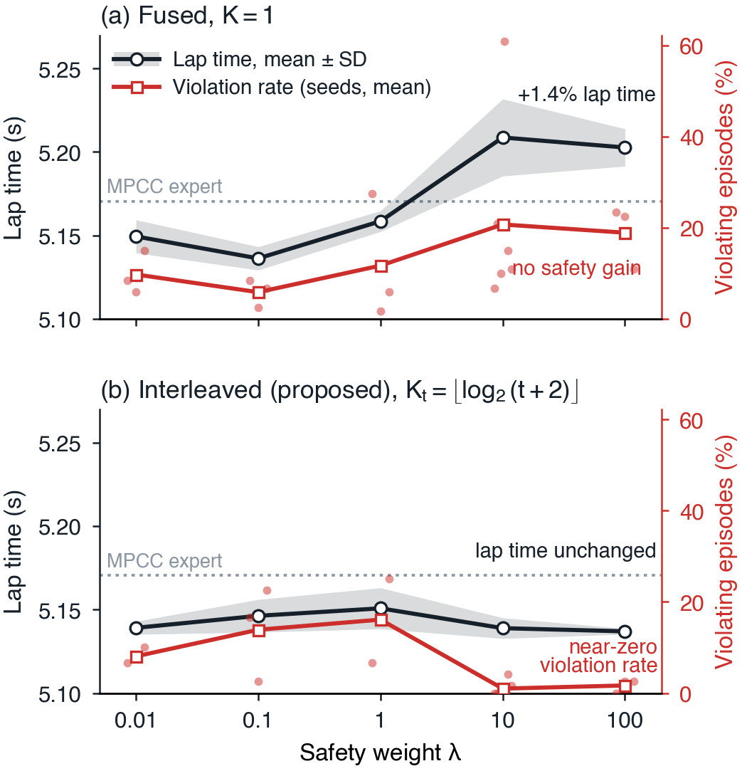
Violating episodes leave the true state bounds in closed loop. Fused training trades safety against optimality through λ, and no weight is safe on every seed within 4000 steps. Every interleaving budget is safe or nearly safe with fewer gradient steps. When corrections are sparse, as with a single-action policy that imitates saturated LQR and needs correction at only 1.5% of states, the step-consistency condition fails and interleaving stalls.

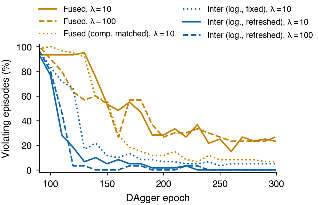
Autonomous racing without a runtime filter

A dynamic bicycle model races on an L-shaped track. A model predictive contouring control (MPCC) expert supplies demonstrations through DAgger. A predictive safety filter supplies the projected actions, during training only.

120 starts per seed 300 DAgger epochs 57 candidate actions per filter call

1.0%violating episodes at λ = 10, against 15.3% for plain behavior cloning

5.139 smean lap time, against 5.144 s for plain behavior cloning and 5.219 s for the filtered expert

~6×fewer violating episodes than fused training at its best weight (λ = 0.1, 5.8%)

Expert trajectories: most laps stay on the track, five episodes leave it. — **Expert**MPCC, no filter
**5.168 s** · 5/40 violating

Filtered expert trajectories: no episode leaves the track. — **Filtered expert**MPCC with a runtime filter
**5.221 s** · 0/40 violating

Fused-penalty trajectories over six seeds: many episodes leave the track, mostly at the corners. — **Fused penalty**One fused step per minibatch
**5.211 s** · 34/240 violating

Compute-matched fused trajectories over six seeds: fewer episodes leave the track than with one fused step, mostly after the hairpin. — **Fused (compute matched)**K_t fused steps per minibatch
**5.193 s** · 11/240 violating

Interleaved trajectories with one safety step per minibatch over six seeds: several episodes leave the track, many at the top-left corner. — **Inter (K = 1)**One safety step per minibatch
**5.143 s** · 18/240 violating

Interleaved trajectories with a logarithmic budget and fixed targets over six seeds: a dozen episodes leave the track. — **Inter (log., fixed)**Logarithmic budget, fixed targets
**5.144 s** · 12/240 violating

Interleaved trajectories over six seeds: a single episode leaves the track. — **Inter (log., refreshed): proposed**Logarithmic budget, refreshed targets
**5.141 s** · 1/240 violating

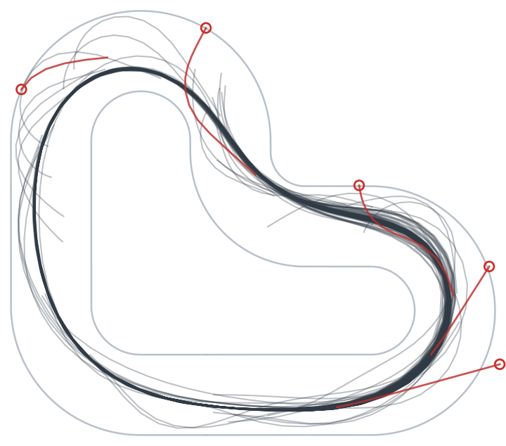
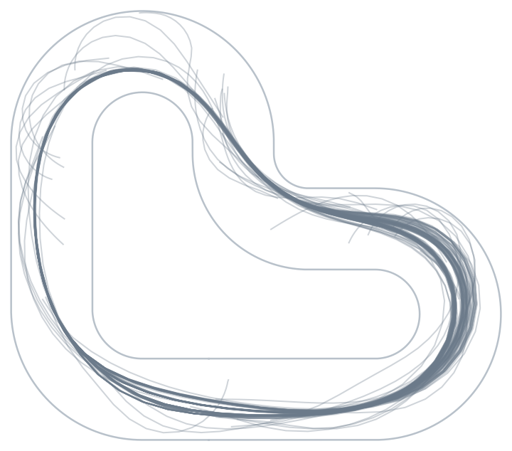
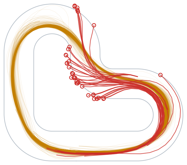
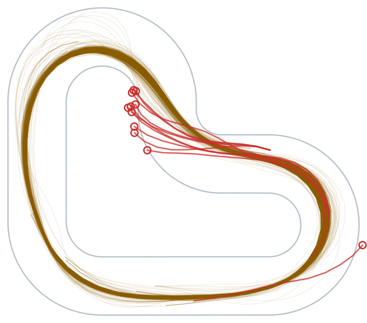
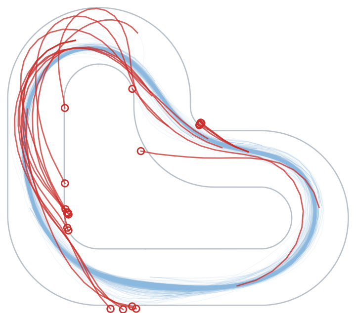
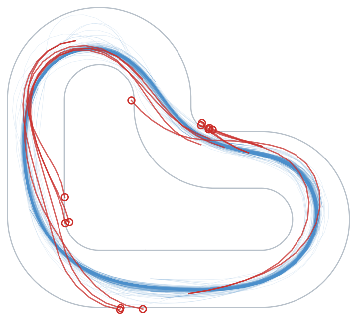
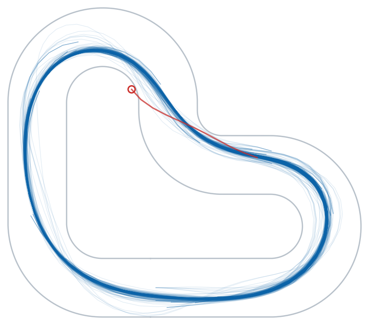
Reading the panels. Closed-loop trajectories from the 40-start illustration bank. The learned policies use six seeds each at λ = 10 and run with no filter; the experts run once.

Each episode is drawn until its first violation; the final 2.5 s before it are red, and the violation is circled. The headline numbers and the table below use the separate 120-start bank.

Ablations at λ = 10

120 starts per seed: six seeds for the middle block, three for the others. Lap time is the mean ± SD of seed-level means. All methods refresh targets except Inter (log., fixed).
Method	Safety updates	Violating episodes	Lap time (s)
Plain BC on raw demonstrations	—	55/360	5.144 ± .002
Plain BC on filtered demonstrations	—	24/360	5.189 ± .007
Fused	1	149/720	5.209 ± .023
Inter (K = 1)	1	84/720	5.142 ± .006
Fused (compute matched)	K_t	41/720	5.192 ± .014
Inter (log., fixed)	K_t	44/720	5.142 ± .006
Inter (log., refreshed)	K_t	7/720	5.139 ± .006
Fused, step η/(1 + λ)	1	271/360	5.336 ± .039
Primal–dual, final λ ≈ 4.4	1	56/360	5.201 ± .009
Primal–dual, final λ ≈ 19	1	46/360	5.178 ± .020
Inter (K = 7)	7	9/360	5.150 ± .020

Lap time and violation rate against the safety weight λ. Fused training slows and does not get safer as λ grows; interleaving keeps its lap time and its violation rate drops to near zero at λ of 10 and above. — Safety weightFor fused training, λ is a trade-off: from 0.1 to 10, laps slow from 5.136 to 5.209 s while violations rise. For interleaving, λ scales the safety step and only sets how quickly violations vanish. Lap times stay within 5.137–5.151 s.

Violating episodes over DAgger epochs. Fused variants stay between 7 and 27 percent late in training; refreshed interleaving reaches zero after epoch 230. — During trainingViolating episodes, evaluated without a filter on ten starts every ten epochs. After epoch 200, fused training still averages 26–27% at λ ∈ {10, 100}, and 9% when compute matched. Refreshed interleaving records none after epoch 230.

Perspective

Separate the objectives.
Keep the filter as a fallback.

Separating task optimization from safety correction turns imitation learning into inexact projected gradient descent in the space of policy outputs. When corrections are dense, the safety steps alone drive the policy toward the constrained optimum.

When corrections are sparse, as in racing, interleaving still yields policies that are safer than penalty-based training at the lap time of unconstrained imitation, with a safety weight that only needs to be large enough.

The guarantees concern the training states, so a runtime filter remains a sensible fallback. Extending them to sparse corrections, through architectures that localize safety updates or safety targets aligned with the expert’s behavior, is left for future work.

Read & build on the work

Read the paper.

The manuscript contains the full analysis with proofs, the planning example, and the racing ablations.

arXiv

Cite this work

Interleaved Projected Gradient Descent for Safe Imitation Learning
Shengfan Cao and Francesco Borrelli

arXiv preprint, 2026.

@misc{cao2026interleaved,
  title         = {Interleaved Projected Gradient Descent
                   for Safe Imitation Learning},
  author        = {Shengfan Cao and Francesco Borrelli},
  year          = {2026},
  eprint        = {2610.07167},
  archivePrefix = {arXiv},
  primaryClass  = {eess.SY},
  url           = {https://arxiv.org/abs/2610.07167}
}

InterleavedProjected Gradient Descent
for Safe Imitation Learning

Can the safety filter make
the policy safer to begin with?

Interleaving against
a fused penalty.

Every safety step
moves every action.